Approximate estimation¶

When $n$ players make exact enumeration infeasible, mllm-shap approximates Shapley-style attributions by sampling coalitions. Three built-in estimators trade budget for accuracy:

MonteCarloEstimator — uniform random coalitions; attributions come from estimand plugins (Shapley or Banzhaf).
ComplementaryEstimator — symmetric pairs $(S, N\setminus S)$ with complementary-contribution (CC) aggregation.
NeymanEstimator — two-phase CC sampling with Neyman allocation over coalition sizes.

Budget model¶

All estimators read ExplainConfig.explanation.budget.fraction in $(0, 1]$. The fraction scales a method-specific maximum:

Estimator	Maximum coalitions
Monte Carlo	$2^n$
Complementary / Neyman	$2^n$ (pairs, so budgets are even)

Every estimator evaluates the empty coalition $\emptyset$ and the grand coalition $N$. Complementary and Neyman samplers yield the pair $(N, \emptyset)$ first, then all $n$ singleton pairs $(\{i\}, N\setminus\{i\})$, so their budget never drops below $2 + 2n$ masks (or $2^n$). For Monte Carlo, ExplainRunner adds whichever boundary coalition the random draws missed. $v(N)$ is scored from the base generation, so it costs no extra backend call.

Monte Carlo and estimand delegation¶

Monte Carlo draws random coalitions and does not embed Shapley weights. Coalition payoffs $v(S)$ are aggregated by the selected estimand plugin:

\[\text{MC} \rightarrow \{v(S_k)\}_{k=1}^{m} \xrightarrow{\text{EstimandAggregator}} (\phi_1, \ldots, \phi_n)\]

The same sampled masks yield different attributions under Shapley vs Banzhaf — a useful sanity check that estimand wiring is correct.

What the aggregator computes from partial samples¶

On a complete table the estimand plugins return the exact value. On a partial sample they estimate it from the observed marginal pairs. Let $P_{i,k}$ be the observed pairs $(S, S\cup\{i\})$ with $i \notin S$ and $|S| = k$, and $K_i$ the coalition sizes with at least one such pair. The Shapley estimate is the stratified mean

\[\hat\phi_i = \frac{n}{|K_i|} \sum_{k \in K_i} \frac{1}{n}\,\overline{\Delta}_{i,k}, \qquad \overline{\Delta}_{i,k} = \frac{1}{|P_{i,k}|}\sum_{S \in P_{i,k}} \big(v(S\cup\{i\}) - v(S)\big)\]

Each size stratum carries Shapley weight $1/n$; sizes without an observed pair are skipped and the sum is rescaled by $n / |K_i|$ so the estimate stays on the scale of the full sum. The Banzhaf estimate uses the same strata with the Banzhaf stratum probabilities $p_k = \binom{n-1}{k} / 2^{n-1}$, renormalized over the observed sizes:

\[\hat\beta_i = \frac{\sum_{k \in K_i} p_k\,\overline{\Delta}_{i,k}} {\sum_{k \in K_i} p_k}\]

It equals the plain mean of all observed marginals only in expectation under uniform sampling of coalitions, where stratum $k$ is hit with probability $p_k$.

Both estimates are consistent (they converge to the exact value as coverage grows) and exact on additive games at any coverage. They are not unbiased for general games at low coverage: a player whose observed pairs fall in a few strata inherits the mean marginal of those strata.

Efficiency, $\sum_i \hat\phi_i = v(N) - v(\emptyset)$, holds exactly only on the full coalition table (exact, or any estimator at budget.fraction: 1.0). Below the full table every estimator here returns values whose sum differs from $v(N) - v(\emptyset)$; the gap shrinks as the budget grows, which the next section measures.

Complementary contributions¶

Complementary sampling evaluates symmetric pairs and accumulates CC statistics in $M_{i,j}$ (how often player $i$ appears in size-$j$ coalitions) and $C_{i,j}$ (summed complementary contributions). For pair $(S, N\setminus S)$ with payoffs $v(S)$ and $v(N\setminus S)$:

\[u = v(S) - v(N\setminus S)\]

Each $u$ updates $C$ for players present in $S$ and $N\setminus S$. Final attributions combine element-wise ratios $C_{i,j}/M_{i,j}$ across coalition sizes:

\[\hat\phi_i = \frac{1}{n} \sum_{j=1}^{n} \frac{C_{i,j}}{M_{i,j}}\]

The column $j = n$ comes only from the pair $(N, \emptyset)$, which is sampled exactly once and contributes $(v(N) - v(\emptyset))/n$ to every player. Without it every player would lose its $S = N\setminus\{i\}$ marginal. Masks are matched to their complements by value, so the aggregation does not depend on the order in which coalitions were evaluated.

A cell with $M_{i,j} = 0$ contributes zero to $\hat\phi_i$. Column $j = 1$ of player $i$ is filled only by the pair $(\{i\}, N\setminus\{i\})$, which a random draw rarely hits, while its partner column $j = n$ is always present. Leaving it empty biases the attribution sum away from $v(N) - v(\emptyset)$. Both samplers therefore evaluate the singleton pairs right after $(N, \emptyset)$ and draw the remaining pairs uniformly at random. On an additive 8-player game at budget.fraction=0.5 the mean attribution sum is within 0.03 of $v(N) - v(\emptyset)$ (it was 1.7 too high without the singleton pairs).

Neyman allocation¶

Neyman-CC extends complementary sampling with two phases:

Initial sampling — after the boundary and singleton pairs, structured draws fill every $M_{i,j}$ cell up to $m_{\text{init}}$ times, capped by the $\binom{n-1}{j-1}$ size-$j$ coalitions that contain player $i$. The grid is walked size by size, round-robin over players, so a short budget leaves the same sizes empty for every player. Phase one ends once every feasible cell is filled or a full pass yields no new coalition.
Neyman allocation — the remaining budget is split across coalition sizes $j \ge \lceil n/2 \rceil$ proportional to estimated standard deviations $\hat\sigma_{i,j}$, never assigning a size more pairs than it has left unsampled. When every variance estimate is zero the remaining pairs are split by the number of unsampled pairs per size.

Variance estimates use the complementary sample variance:

\[\hat\sigma^2_{i,j} = \frac{1}{M_{i,j}-1} \left(\sum u^2 - \frac{(\sum u)^2}{M_{i,j}}\right)\]

Allocation follows the Neyman rule (symmetric halves summed):

\[\hat M_j \propto \sqrt{ \sum_{i} \frac{\hat\sigma^2_{i,j}}{j+1} + \sum_{i} \frac{\hat\sigma^2_{i,n-j}}{n-j+1} }\]

where $n - j$ is the size of the complement of a size-$j$ coalition.

Small budgets: phase one may consume the whole allowance before allocation begins, and then behaves like complementary sampling with structured draws. On the 8-player game below both reach a mean relative L1 error of 0.55 at budget.fraction=0.1 over 200 seeds; that is an observation, not a guarantee.

Because allocation depends on phase-one payoffs, Neyman requires a two-step API: sample_masks() (phase one), begin_allocation(), then sample_allocation_masks(). ExplainRunner runs both phases: any estimator that implements TwoPhaseEstimator gets its phase-one payoffs and a second scheduling pass for the allocated masks.

Choosing a budget¶

Convergence depends on the game, so the numbers below illustrate rather than guarantee. The snippet builds an eight-player game with additive weights and two interactions and computes the exact Shapley values from all 256 coalitions. It reports each estimator’s mean relative L1 error $\sum_i |\hat\phi_i - \phi_i| / \sum_i |\phi_i|$ over five seeds as the budget fraction grows, adding the boundary coalitions as ExplainRunner does.

import matplotlib.pyplot as plt
import numpy as np

from mllm_shap import (
    CoalitionMask,
    ComplementaryEstimator,
    ExactEstimator,
    MonteCarloEstimator,
    NeymanEstimator,
    PlayerSet,
    ShapleyAggregator,
)

n = 8
players = PlayerSet(player_ids=tuple(f"p{i}" for i in range(n)))
weights = np.random.default_rng(0).normal(size=n)

def payoff(mask: CoalitionMask) -> float:
    present = np.array(mask.present)
    pair_bonus = 1.5 if present[0] and present[1] else 0.0
    crowding = -1.0 if present[2:5].sum() >= 2 else 0.0
    return float(weights @ present) + pair_bonus + crowding

def estimate(estimator, fraction: float, seed: int) -> np.ndarray:
    masks = list(estimator.sample_masks(players, fraction, False, seed))
    payoffs = [payoff(mask) for mask in masks]
    if isinstance(estimator, NeymanEstimator):
        estimator.begin_allocation(masks, payoffs)
        extra = list(estimator.sample_allocation_masks())
        masks += extra
        payoffs += [payoff(mask) for mask in extra]
    seen = {mask.present for mask in masks}
    for present in ((True,) * n, (False,) * n):
        if present not in seen:
            masks.append(CoalitionMask.from_sequence(present))
            payoffs.append(payoff(masks[-1]))
    aggregator = ShapleyAggregator()
    return np.array(estimator.estimate_attributions(masks, payoffs, aggregator))

exact = estimate(ExactEstimator(), 1.0, 0)
fractions = (0.1, 0.2, 0.3, 0.5, 0.75)
estimators = {
    "Monte Carlo": MonteCarloEstimator,
    "Complementary": ComplementaryEstimator,
    "Neyman-CC": NeymanEstimator,
}
errors = {
    name: [
        np.mean([
            np.abs(estimate(make(), fraction, seed) - exact).sum()
            / np.abs(exact).sum()
            for seed in range(5)
        ])
        for fraction in fractions
    ]
    for name, make in estimators.items()
}

print("fraction " + " ".join(f"{name:>13}" for name in errors))
for index, fraction in enumerate(fractions):
    row = " ".join(f"{errors[name][index]:>13.3f}" for name in errors)
    print(f"{fraction:>8} {row}")

figure, axis = plt.subplots(figsize=(6, 3.5))
for name, values in errors.items():
    axis.plot(fractions, values, marker="o", label=name)
axis.set_xlabel("budget fraction")
axis.set_ylabel("relative L1 error")
axis.legend()

Mean relative L1 error over five seeds

fraction   Monte Carlo Complementary     Neyman-CC
1         0.564         0.509         0.538
2         0.228         0.406         0.381
3         0.140         0.267         0.223
5         0.096         0.157         0.134
75         0.054         0.074         0.079

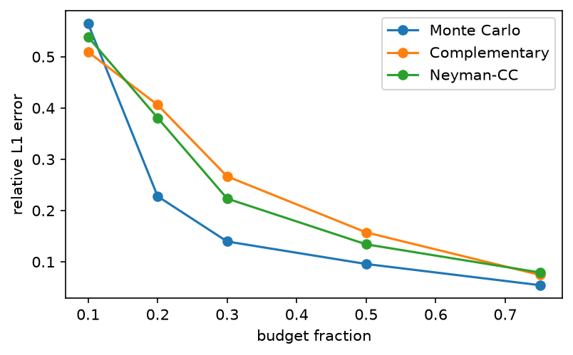
$Relative L1 error of three estimators against the budget fraction$

On this game Monte Carlo with the stratified Shapley aggregator converges fastest. Neyman-CC catches up once the budget leaves room for its second phase; at low budgets it behaves like complementary sampling. Before fixing a budget for an expensive backend, run the same comparison on a game that resembles your prompts, or on the prompt itself with a cheap backend and exact as the reference. examples/estimator_comparison.ipynb goes further.

References¶

Zhang, J., Sun, Q., Liu, J., Xiong, L., Pei, J., Ren, K. (2023). Efficient Sampling Approaches to Shapley Value Approximation. Proc. ACM Manag. Data 1(1). https://doi.org/10.1145/3588728
Neyman, J. (1934). On the Two Different Aspects of the Representative Method. J. R. Stat. Soc. 97(4). https://doi.org/10.2307/2342192
Castro, J., Gómez, D., Tejada, J. (2009). Polynomial calculation of the Shapley value based on sampling. Comput. Oper. Res. 36(5). https://doi.org/10.1016/j.cor.2008.04.004
Mitchell, R., Cooper, J., Frank, E., Holmes, G. (2022). Sampling Permutations for Shapley Value Estimation. Journal of Machine Learning Research 23(43).
Goldshmidt, R., Horovicz, M. (2024). TokenSHAP: Interpreting Large Language Models with Monte Carlo Shapley Value Estimation. arXiv:2407.10114. https://arxiv.org/abs/2407.10114

Estimator	Maximum coalitions
Monte Carlo	\(2^n\)
Complementary / Neyman	\(2^n\) (pairs, so budgets are even)